Table of Contents

This is part 3 of a 4-part series (part 1: Euler's formula and Fourier series; part 2: the DFT, FFT, and spectral methods). Figures and the trained model are reproducible from the repo: pixi run wno-train, then pixi run figs-post3.

Fourier's blind spot

A Fourier coefficient is an integral over all time. The basis function $e^{i\omega t}$ has perfect frequency and no location — it rings forever. So a spectrum answers "what frequencies are present?" but is structurally incapable of answering "when?" A drum hit at $t = 3\,\mathrm{s}$ and the same hit at $t = 30\,\mathrm{s}$ have the same magnitude spectrum; all the timing hides in the phase, scrambled across every coefficient.

Part 2's fix was the spectrogram: window the signal, transform each slice. But the window length is a contract you sign in advance. Take a signal with both a slow chirp and a 2-millisecond click, and no single window serves both clients:

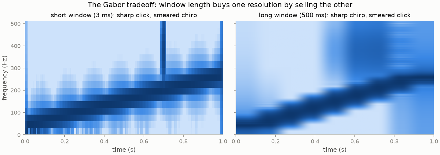
This isn't an engineering failure; it's a theorem. Gabor's uncertainty principle — the same inequality as Heisenberg's, applied to a signal and its transform — bounds the product of time spread and frequency spread:

$$ \Delta t \cdot \Delta \omega \ge \frac{1}{2}. $$

You cannot beat the bound. What you can do is spend it differently at different frequencies — and that observation is the whole wavelet idea.

Wavelets: constant-Q tiling

High-frequency events are typically brief (clicks, edges, shocks); low-frequency behavior is typically long (drones, trends). So instead of one fixed window, take one oscillating bump $\psi$ — the mother wavelet — and generate a family by scaling and translating it:

$$ \psi_{a,b}(t) = \frac{1}{\sqrt{a}}\, \psi\!\left(\frac{t - b}{a}\right). $$

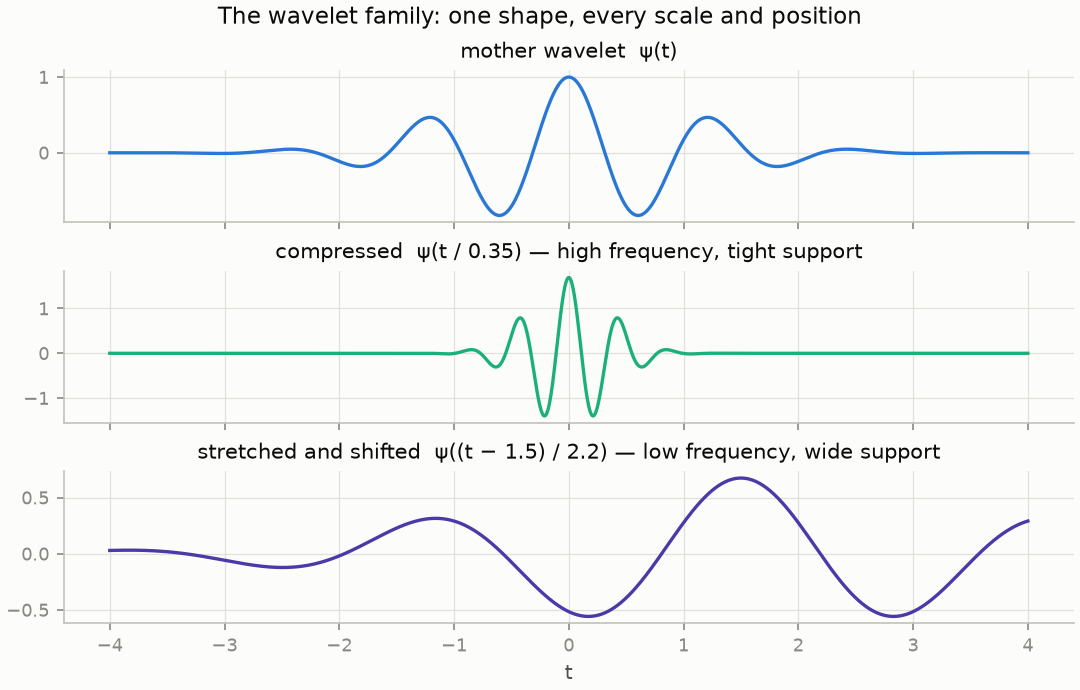
The continuous wavelet transform correlates the signal against every member of the family:

$$ W(a, b) = \int_{-\infty}^{\infty} f(t)\, \frac{1}{\sqrt{a}}\, \overline{\psi\!\left(\frac{t-b}{a}\right)} dt . $$

Small scale $a$ = a short, high-frequency probe with fine time resolution; large $a$ = a long, low-frequency probe with fine frequency resolution. Every tile in the time-frequency plane has the same relative bandwidth (musicians: each octave gets equal treatment — "constant-Q"). Mechanically it's just template matching, a convolution per scale:

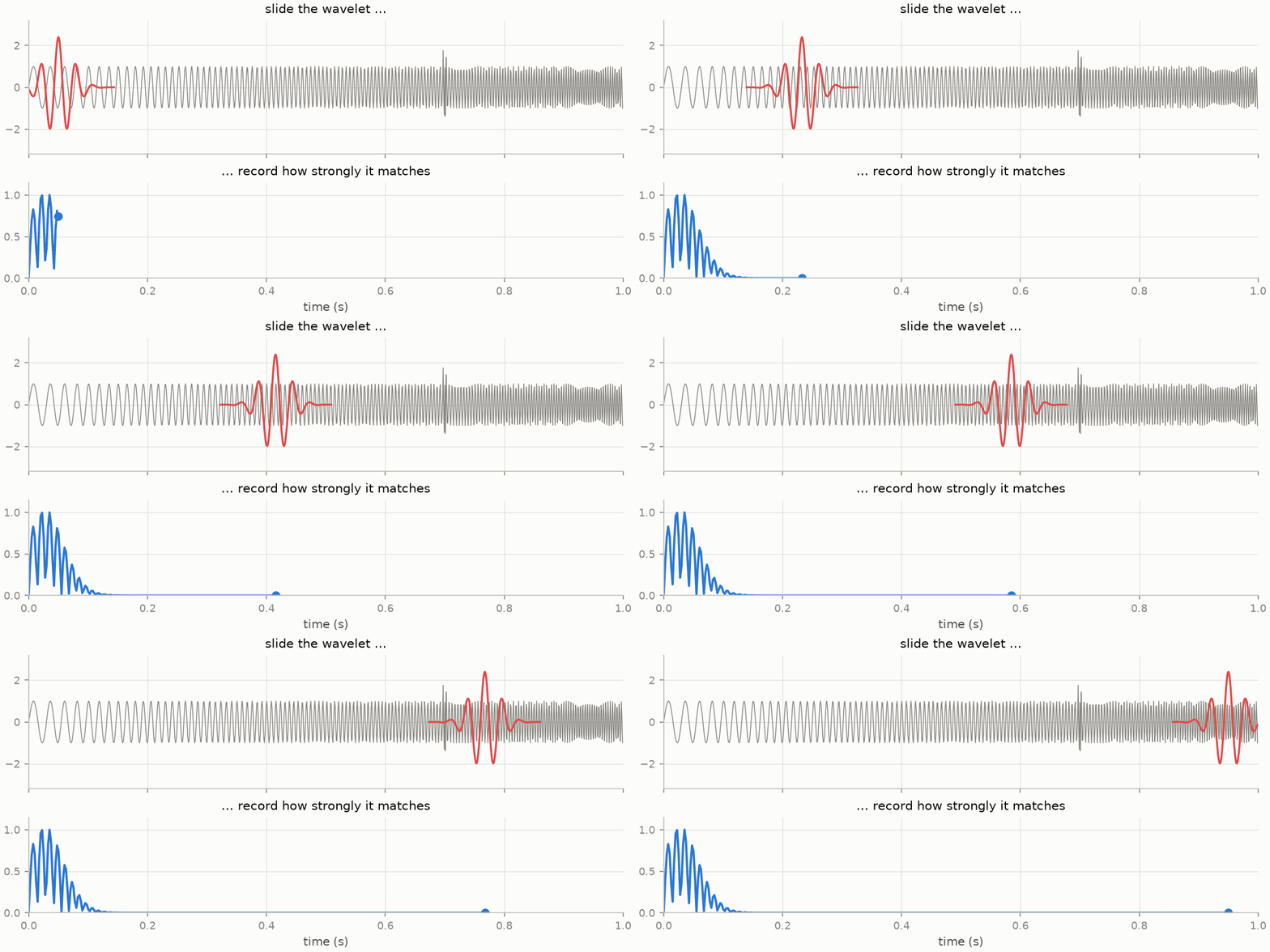
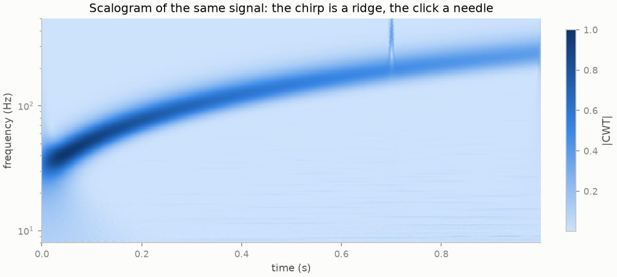
Stack the responses at all scales and you get the scalogram. Same chirp-plus-click signal as above — now the chirp is a crisp ridge and the click is a needle, localized to milliseconds at high frequency where short probes live:

(The only real constraint on $\psi$ is the admissibility condition — zero mean and finite $\int |\hat\psi(\omega)|^2 / |\omega|\, d\omega$ — i.e., it must actually wave.)

The DWT: Mallat's pyramid

The CWT is gloriously redundant — a whole 2D picture from a 1D signal. For computation you want the opposite: a basis. Mallat and Daubechies showed you can choose scales $a = 2^j$ and shifts $b = k \cdot 2^j$ and, for the right $\psi$, get an orthonormal basis — no information lost, none duplicated. Daubechies' families (db2, db3, db4...) are compactly supported: each basis function touches only a few samples.

The algorithm is a two-channel filter bank. Convolve with a lowpass filter $h$ and a highpass filter $g$, downsample each by 2 (safe because the filters halved the band — part 2's aliasing lesson), then recurse on the lowpass half:

$$ x \longrightarrow (\,\mathrm{cA}_1, \mathrm{cD}_1\,) \longrightarrow (\,\mathrm{cA}_2, \mathrm{cD}_2, \mathrm{cD}_1\,) \longrightarrow \cdots $$

Each level splits off the finest remaining detail. For $N$ samples the whole pyramid costs $O(N)$ — faster than the FFT. Here it is run on a signal with a slow wave, a step, and a spike, using the simplest wavelet (Haar: average and difference):

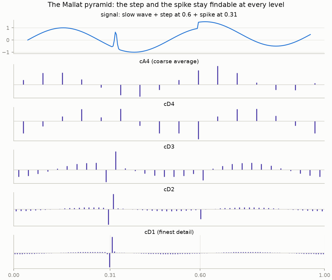
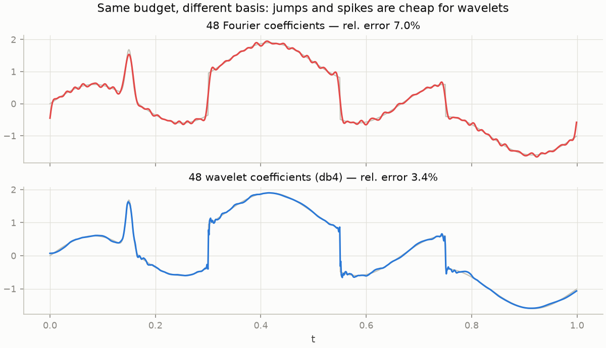
The point to stare at: the spike and the step stay findable at every level — a handful of large coefficients sitting at the right location. A Fourier basis would democratically smear them across all frequencies. This is Fourier's Gibbs problem from part 1, solved by changing basis. The consequence is sparsity, and it's why this transform runs your world quietly: JPEG 2000 compresses images with it, denoisers threshold small wavelet coefficients (Donoho's soft thresholding), and FBI fingerprints live in a wavelet format. A budget of 48 coefficients makes the argument concisely:

(The formal scaffolding behind this — multiresolution analysis — is a nested ladder of approximation spaces $V_0 \subset V_1 \subset \cdots$ with $V{j+1} = V_j \oplus W_j$; the wavelets span the detail spaces $W_j$. Mallat's book has the full story.)_

Neural operators in one section

Now the modern part. Classical networks learn functions between finite-dimensional spaces. An operator maps functions to functions — like "initial condition $\mapsto$ PDE solution at time $T$", which is exactly the map we solved numerically in part 2's spectral-methods section. Operator learning trains a network $G_\theta : u_0(\cdot) \mapsto u(\cdot, T)$ once, then evaluates it in microseconds per new input — a surrogate solver. Done right it is discretization-invariant: the same weights work at any grid resolution, because the layers act on functions, not pixel vectors.

The Fourier Neural Operator (Li et al., 2020) builds the layer from part 2's three-step spectral pattern — transform, act diagonally, transform back — with the diagonal action learned:

$$ v_{\mathrm{out}} = \sigma\Big( \mathcal{F}^{-1}\big( R_\theta \cdot \mathcal{F} v \big) + W v + b \Big), $$

where $\mathcal{F}$ is the FFT along the spatial axis, $R_\theta$ holds learnable complex weights on the lowest $k$ modes (the rest truncated to zero), and $W v + b$ is a pointwise skip connection that carries what the truncation drops. Compare: heat flow multiplied mode $k$ by $e^{-\nu k^2 t}$; the FNO multiplies mode $k$ by whatever the data says. It's a learnable spectral method.

But an FFT-based layer inherits Fourier's blind spot. Global modes are a clumsy language for sharp fronts and shocks — precisely what nonlinear PDEs love to produce. You know the remedy from the last two sections: swap the transform. The Wavelet Neural Operator (Tripura & Chakraborty, 2022) keeps the recipe and replaces $\mathcal{F}$ with the DWT, putting the learnable weights on wavelet subbands:

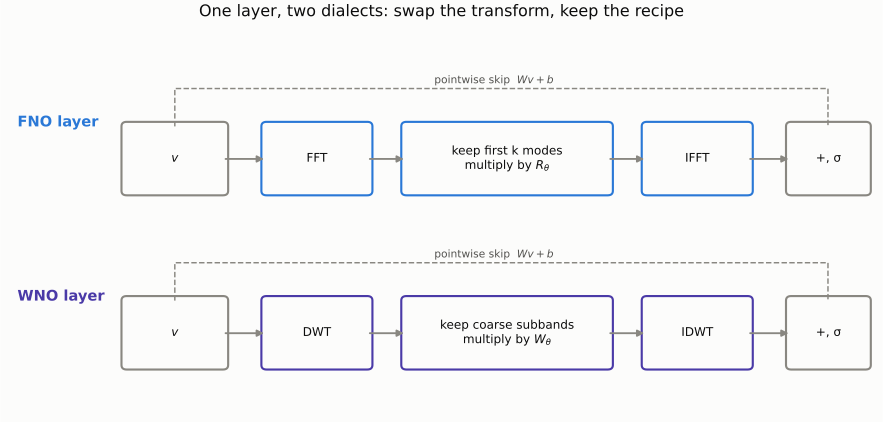
Because wavelet coefficients are localized, the learned kernel can treat a front at $x = 0.3$ differently from smooth flow at $x = 0.7$ — spatial adaptivity that global Fourier modes can't express. Empirically WNOs hold up better on sharp-gradient, non-periodic, and boundary-dominated problems.

A minimal WNO in JAX

Everything below is in the repo under src/ftx/wno/ — four short files, pure JAX plus jaxwt for a differentiable DWT.

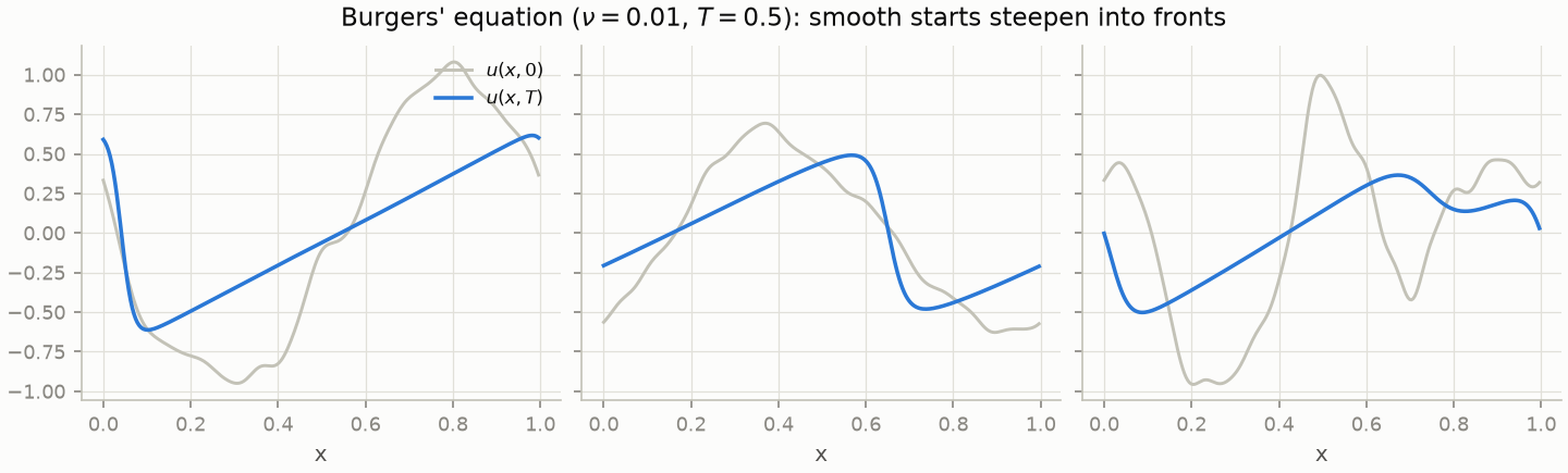
The problem. Viscous Burgers' equation on the periodic unit interval — the classic toy for "smooth in, sharp out":

$$ \frac{\partial u}{\partial t} + u \frac{\partial u}{\partial x} = \nu \frac{\partial^2 u}{\partial x^2}, \qquad \nu = 0.01 . $$

Learn the operator $u(\cdot, 0) \mapsto u(\cdot, 0.5)$ on a 256-point grid.

The data is part 2 made executable: 1,128 random smooth initial conditions (Fourier coefficients with $1/k^2$ amplitudes), each integrated pseudo-spectrally — derivatives via rfft/irfft, 2/3-rule dealiasing, integrating-factor RK4 so the stiff diffusion term is handled exactly. jax.vmap over samples, jax.lax.scan over time; the whole dataset generates in seconds on a CPU. The advection term steepens every smooth start into fronts:

The model is three WNO blocks between a lift and a projection:

def _wno_block(p, v):                      # v: (batch, n, width)
    batch, n, width = v.shape
    vc = v.transpose(0, 2, 1).reshape(batch * width, n)
    coeffs = dwt(vc)                       # jaxwt.wavedec, db4, 4 levels
    out = []
    for i, c in enumerate(coeffs):
        c = c.reshape(batch, width, -1)
        if i < len(p["spectral"]):         # coarsest 3 subbands: learnable
            y = jnp.einsum("bcl,lco->bol", c, p["spectral"][i])
        else:                              # finest details: truncated
            y = jnp.zeros_like(c)
        out.append(y.reshape(batch * width, -1))
    wave = idwt(out, n).reshape(batch, width, n).transpose(0, 2, 1)
    return jax.nn.gelu(wave + v @ p["skip"]["w"] + p["skip"]["b"])

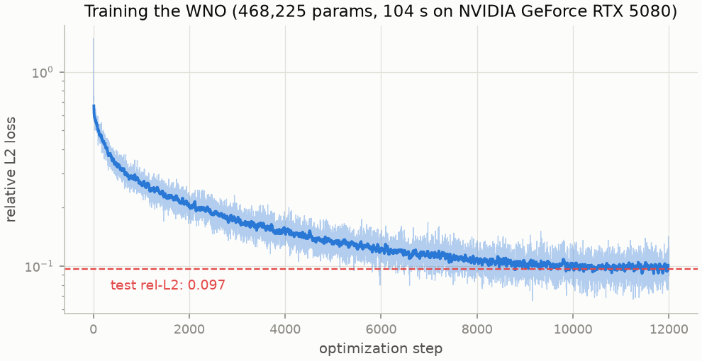
That einsum is the exact analogue of the FNO's $R_\theta$: an independent learnable channel-mixing matrix per wavelet coefficient, applied only on the coarse subbands. Parameters live in a plain pytree dict; no framework. Training is optax.adam on the relative L2 loss $\lVert \hat{u} - u \rVert_2 / \lVert u \rVert_2$ — 104 seconds on an RTX 5080, about 5–6 minutes on a CPU. (The wall-clock gap understates the hardware difference: per training step the GPU is 5.6× faster, and ~40× on batched inference — pixi run wno-bench, analyzed in part 4. This loop fetches the loss to host every step for logging, which stalls the GPU; the run's device is recorded in metrics.json.) The repo ships a pixi cuda environment (JAX + CUDA 12 on WSL2).

One training trick earns its sentence. Burgers on a periodic domain is translation-equivariant — shift the initial condition, the solution shifts with it — but the DWT is not shift-invariant (unlike the FFT, whose modes just pick up a phase). The model can't inherit the symmetry from its architecture, so we teach it by augmentation: every batch applies a random circular shift to each input-output pair. In our runs this one change cut test error by a third and closed the train-test gap almost entirely:

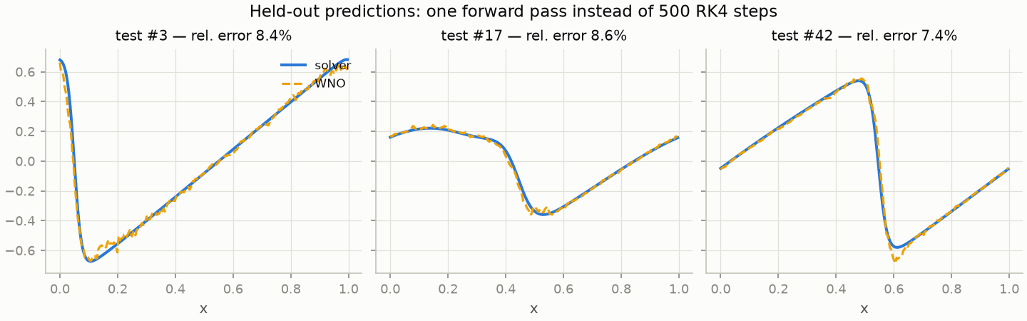
A model this small, trained for minutes, won't match the sub-1% errors of full-size neural operators — the published WNO uses wider channels, more levels, and longer training. What the demo is for: every conceptual ingredient — DWT in, learned weights on coefficients, IDWT out, one forward pass replacing 500 solver steps — in a few hundred lines you can read in one sitting.

When to reach for which

• FFT / spectral methods — periodic, smooth, global structure. Unbeatable when they apply, and they come with 200 years of theory.
• STFT / spectrogram — you need "when and what frequency" and a fixed resolution contract is acceptable (audio, vibration monitoring).
• DWT / wavelets — transients, edges, jumps, multiscale structure; when you want sparsity (compression, denoising) or $O(N)$ speed.
• FNO — learning solution operators for smooth, periodic PDE families fast.
• WNO — same game with shocks, sharp gradients, non-periodic boundaries, or signals whose action is localized.

The through-line of all three posts is one move, inherited from a rejected 1807 memoir: find the basis that makes your operator simple, act there, and come back. Euler's formula supplied the basis; the FFT made the round trip cheap; wavelets rebuilt the basis for a world with edges; and neural operators let the data choose what to do in the middle.

Further reading

• Mallat, A Wavelet Tour of Signal Processing — the reference. His 1989 multiresolution paper is where the pyramid algorithm comes from.
• Daubechies, Ten Lectures on Wavelets — where db4 comes from, building on her 1988 construction of compactly supported orthonormal wavelets.
• Li et al., "Fourier Neural Operator for Parametric PDEs" (2020).
• Tripura & Chakraborty, "Wavelet Neural Operator for solving parametric PDEs" (2022).
• Kovachki et al., "Neural Operator: Learning Maps Between Function Spaces" (2021) — the general theory.
• Hu et al., "Wavelet Diffusion Neural Operator" (2024) — the generative sequel: diffusion models run in wavelet space over whole trajectories, for simulation and control. Now the subject of part 4.