From Series to Samples: the DFT, the FFT, and Why Convolution Is Multiplication

Posted on 2026-07-03 :: Tags: math, fourier, python, jax, scientific-computing

This is part 2 of a 4-part series (part 1 covered Euler's formula and Fourier series). Every figure is generated by deterministic scripts — pixi run figs-post2 reproduces this page.

Discretizing: the DFT is a matrix

Computers don't integrate; they sum. Sample a signal at $N$ points and the Fourier series coefficients from part 1 become the discrete Fourier transform:

$$ X_k = \sum_{n=0}^{N-1} x_n\, e^{-2\pi i\, k n / N}, \qquad x_n = \frac{1}{N}\sum_{k=0}^{N-1} X_k\, e^{+2\pi i\, k n / N}. $$

Everything is built from one complex number, $\omega = e^{2\pi i / N}$ — a single click of a clock hand with $N$ positions. Its powers are the $N$-th roots of unity, and they are the DFT's entire alphabet:

The 16th roots of unity arranged on the unit circle

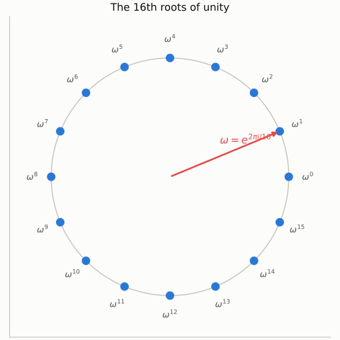
Because the sum is finite, the DFT is literally a matrix-vector product $X = W x$ with $W_{k n} = \omega^{-k n}$. Row $k$ of the matrix is a phasor spinning $k$ times around the circle, sampled $N$ times — you can see the frequencies rise as you read downward:

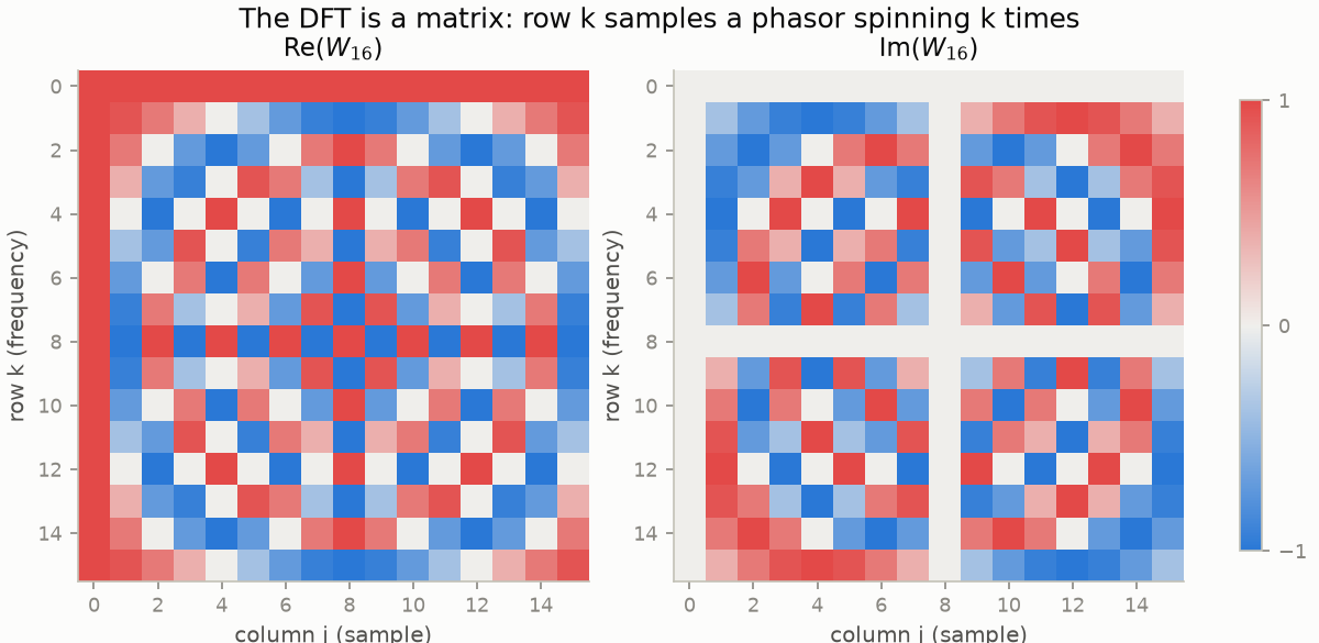
Real and imaginary parts of the 16-point DFT matrix

The orthogonality of complex exponentials survives discretization exactly: $W^* W = N I$, so $W/\sqrt{N}$ is unitary. The DFT is a rigid rotation of $\mathbb{C}^N$ — no information created or destroyed, just re-expressed. Parseval's theorem ($\sum |x_n|^2 = \frac{1}{N}\sum |X_k|^2$) is nothing more than "rotations preserve length."

One more consequence of the matrix view, and it's a fun one. Applying the transform twice gives $W^2 = N \cdot P$, where $P$ reverses indices circularly:

$$ \mathrm{FFT}(\mathrm{FFT}(x))[n] = N\, x[(-n)\ \mathrm{mod}\ N]. $$

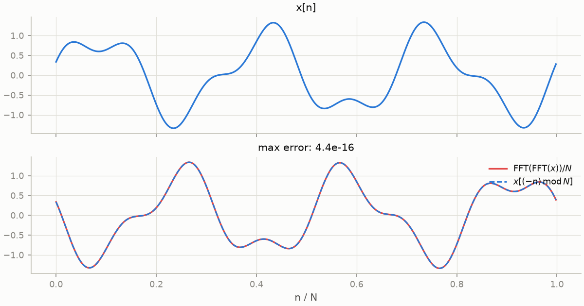
FFT of an FFT: the signal comes back reversed and scaled by N

So $W^4 = N^2 I$: four FFTs bring you home. That forces the eigenvalues of $W/\sqrt{N}$ to be fourth roots of unity, $\lbrace 1, i, -1, -i \rbrace$ — the same reason the continuous transform has the Gaussian and Hermite functions as eigenfunctions. The DFT isn't just like a rotation; it's very nearly a quarter-turn.

Sampling has a speed limit

Discretizing costs something, and the price is paid at high frequency. At a sampling rate $f_s$, the frequencies $f$ and $f + f_s$ produce identical samples — on the roots-of-unity clock, spinning $k$ clicks per step is indistinguishable from $k + N$. Two genuinely different sinusoids, one set of samples:

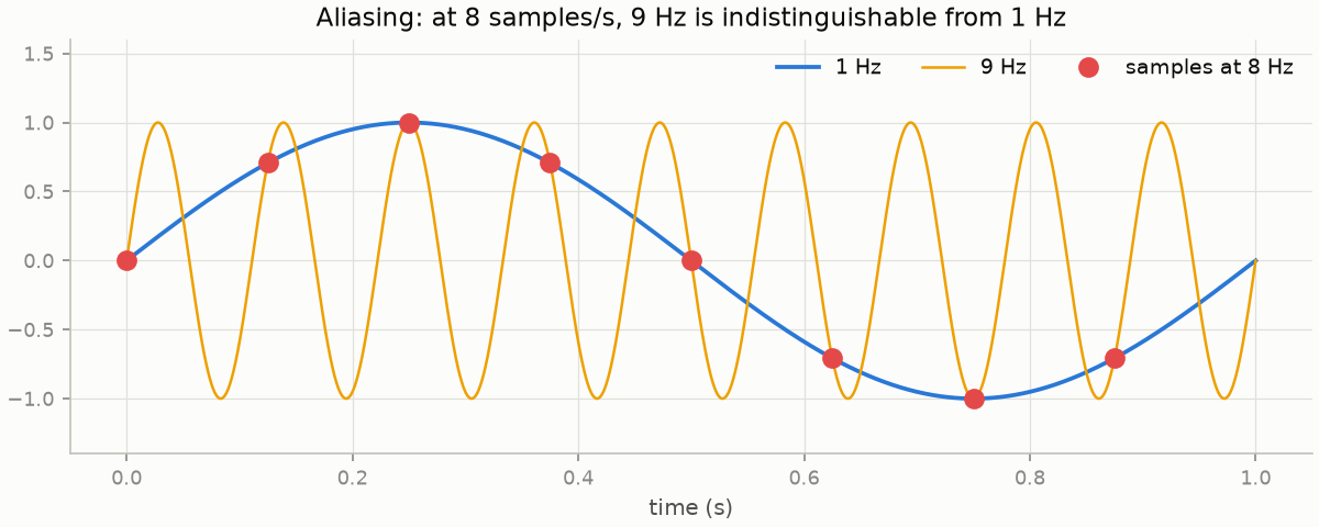
A 1 Hz and a 9 Hz sinusoid passing through the same samples taken at 8 Hz

The Nyquist–Shannon theorem draws the line: a signal containing frequencies only below $f_s / 2$ is exactly recoverable from its samples. Push past it and frequencies fold back down like a reflected ruler — a tone sweeping upward past Nyquist appears to bounce off the ceiling and descend:

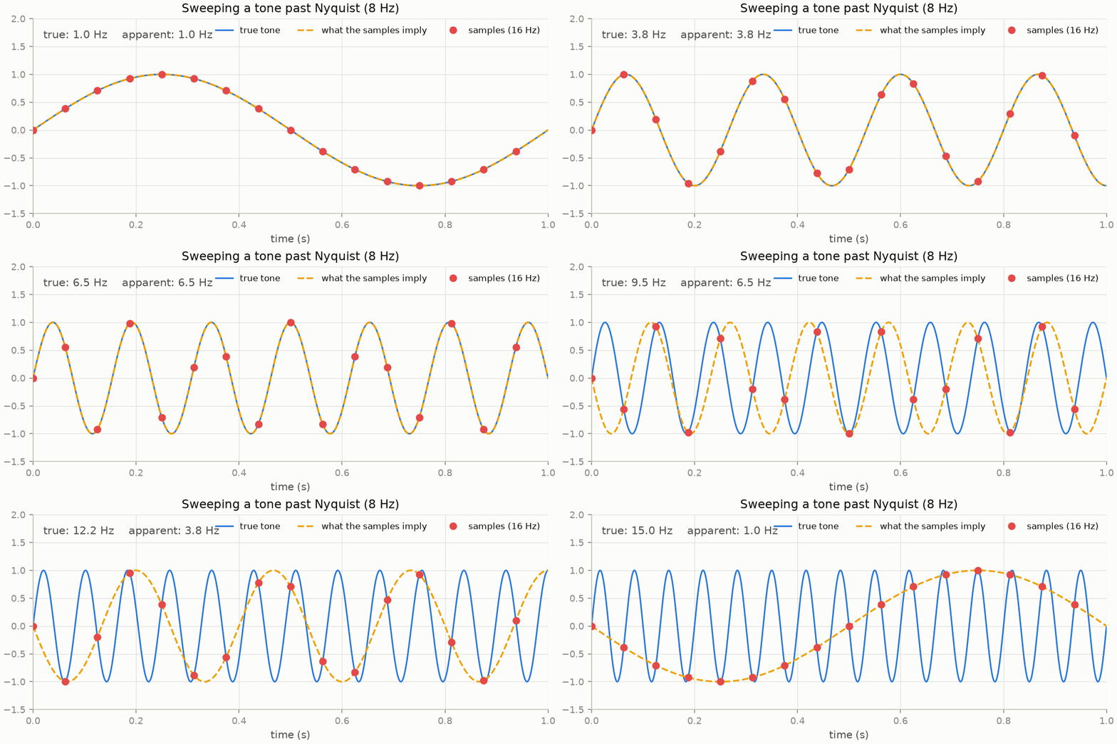
A tone sweeping past the Nyquist frequency and folding back down

This is why anti-aliasing filters sit in front of every analog-to-digital converter, why wagon wheels spin backwards in westerns, and — foreshadowing part 3 — why the "downsample by 2" step inside a wavelet transform must be paired with a filter that removes the top half-band first.

The FFT: divide, conquer, and a footnote from Gauss

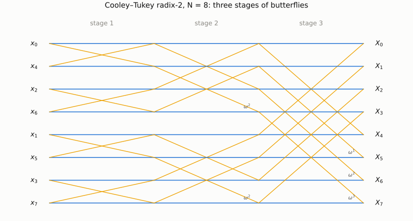
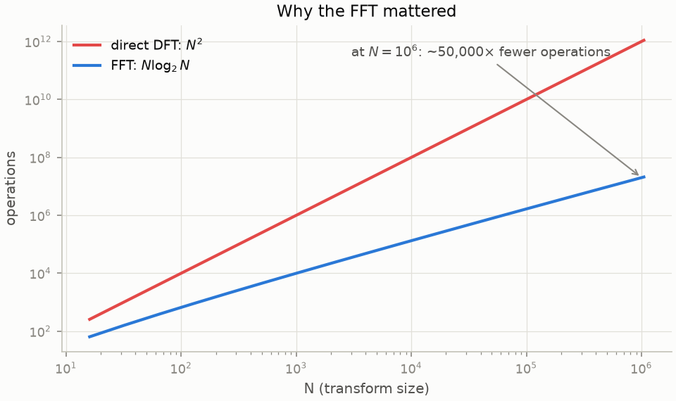
Multiplying by $W$ costs $O(N^2)$. The fast Fourier transform computes the same $X$ in $O(N \log N)$ by exploiting the clock's symmetry. Split the sum into even and odd samples:

$$ X_k = \underbrace{\sum_m x_{2m}\, \omega^{-2mk}}_{E_k} \;+\; \omega^{-k} \underbrace{\sum_m x_{2m+1}\, \omega^{-2mk}}_{O_k} $$

Both halves are themselves DFTs of size $N/2$, and — the crucial bit — the second half of the output reuses them with only a sign flip: $X_{k + N/2} = E_k - \omega^{-k} O_k$. Two half-size problems plus $O(N)$ glue:

$$ T(N) = 2\,T(N/2) + O(N) \implies T(N) = O(N \log_2 N). $$

Unrolled, the recursion becomes $\log_2 N$ stages of "butterfly" operations:

Signal-flow graph of the radix-2 FFT for N = 8

The asymptotic gap is not academic:

Operation counts: N squared versus N log N

Cooley and Tukey published in 1965, motivated in part by detecting Soviet nuclear tests from seismometer data — a problem where transforms of long records had to be feasible. Gauss had the same algorithm in an unpublished 1805 notebook, two years before Fourier's memoir, for interpolating asteroid orbits. It was rediscovered because it was needed; the lesson about publishing your tricks writes itself.

The convolution theorem: the workhorse

Here is the identity that makes the FFT an engine rather than a curiosity. Convolution blends one sequence with another:

$$ (x * y)[n] = \sum_m x[m]\, y[n - m] $$

— it's the operation behind moving averages, filters, blurs, echoes, polynomial multiplication, and probability distributions of sums. Computed directly it costs $O(N^2)$. But in the frequency domain it collapses to pointwise multiplication:

$$ \mathrm{DFT}(x * y) = \mathrm{DFT}(x) \cdot \mathrm{DFT}(y). $$

The proof is two lines with the geometric series and worth doing once by hand: substitute the definition, swap the sums, and the roots-of-unity orthogonality does the rest. So the fast recipe for any convolution is: transform ($N \log N$), multiply ($N$), transform back ($N \log N$).

Watch it do probability. A die is a probability vector; the sum of $k$ dice is that vector convolved with itself $k$ times, i.e. one FFT, a $k$-th power, one inverse FFT. The central limit theorem materializes in front of you:

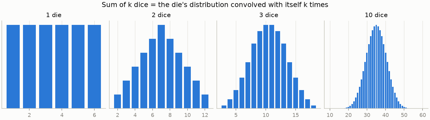
Distributions of sums of 1, 2, 3, and 10 dice computed by FFT convolution

(One care: the DFT's convolution is circular — index arithmetic wraps mod $N$, like everything on the clock. For a linear convolution you zero-pad both inputs to the full output length first. The same trick multiplies million-digit integers: digits are polynomial coefficients, and carrying is a post-processing step.)

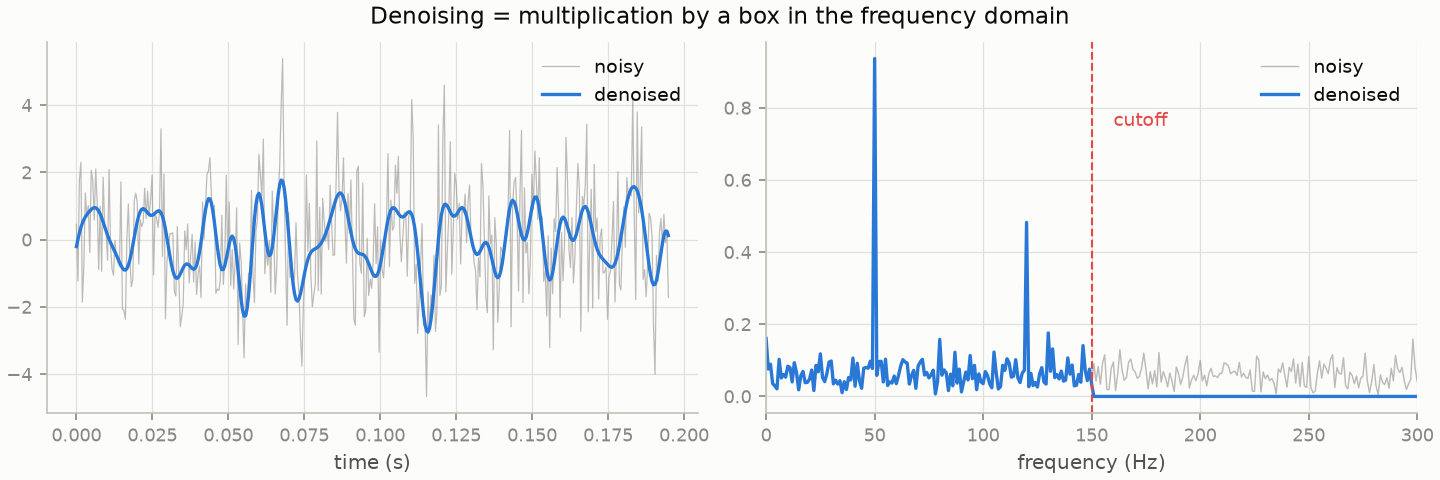
Filtering is the same theorem run for its own sake. Part 1's denoising demo — two tones buried in noise — is just: FFT, zero every bin above 150 Hz, inverse FFT. Multiplication by a box in frequency is convolution with a sinc in time:

FFT denoising of two tones buried in noise

Windows, leakage, and hearing a song

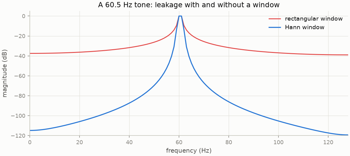
Real signals aren't periodic, but the DFT stubbornly assumes its input is one period of something that repeats. Chop a sine wave mid-cycle and the wraparound jump smears energy across every bin — spectral leakage. The fix is to fade the edges with a window (Hann, Hamming, Blackman...) before transforming, trading a slightly wider peak for enormously quieter sidelobes:

Spectrum of an off-bin tone with a rectangular window versus a Hann window

Slide a window along a long recording, FFT each hop, stack the columns, and you get the short-time Fourier transform — the spectrogram, time-frequency currency of speech, audio ML, and seismology. Here's one of the mp3s sitting in this repo's data/ folder:

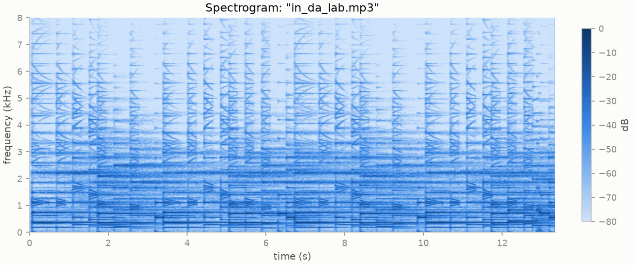
Spectrogram of a hip-hop track showing kick drums, bass, and hi-hats

Kicks are the vertical full-band stripes, the bassline lives in the dark band under 1 kHz, hi-hats sparkle up top. Note the trade you've silently accepted: each column knows roughly when, each row roughly what frequency, and the window length sets the exchange rate. You cannot sharpen both at once — that tension is the opening argument of part 3.

Spectral methods: differentiation becomes multiplication

The eigenfunction fact from part 1 — differentiating $e^{ikx}$ multiplies it by $ik$ — turns the FFT into a numerical-analysis power tool. To differentiate a periodic function: transform, multiply bin $k$ by $ik$, transform back. No stencils, no truncation order — the accuracy is limited only by how fast the function's Fourier coefficients decay. For smooth functions that decay is exponential, and the resulting spectral accuracy embarrasses finite differences:

Convergence of spectral differentiation versus 2nd and 4th order finite differences

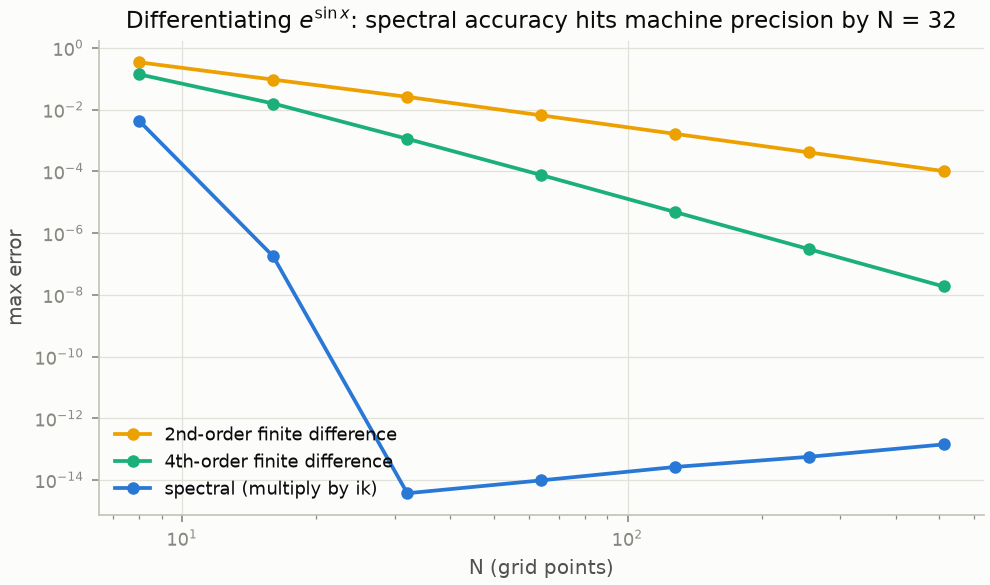
The 2nd-order stencil buys you $h^2$; doubling the grid earns two bits of accuracy. The spectral derivative of $e^{\sin x}$ hits machine precision at $N = 32$ and stays there. This is the engine of pseudo-spectral PDE solvers: in part 3, the Burgers' equation data for training a neural operator is generated exactly this way — derivatives by $ik$ multiplication in Fourier space, time-stepping in physical space.

Two complex-analysis footnotes deserve a sentence each, because they reappear everywhere. First, the DFT is the z-transform $X(z) = \sum x_n z^{-n}$ evaluated at $N$ points on the unit circle — digital filter design is complex analysis on that circle, poles inside for stability. Second, evaluating a polynomial on the roots of unity is exactly what the FFT does, which is why it multiplies polynomials fast — and evaluating a Laurent series on the circle connects the decay rate of Fourier coefficients to the width of the strip where the function is analytic. Smoothness in one domain is decay in the other, in both directions.

Where this goes

The spectral pattern is always the same three-step: transform, act diagonally, transform back. Denoising: zero some bins. Differentiation: multiply by $ik$. Heat flow: multiply by $e^{-\nu k^2 t}$. In part 3 we meet the version where the diagonal action is learned from data — a Fourier neural operator — then swap the FFT for a wavelet transform to get localization in both time and frequency, and train a wavelet neural operator on Burgers' equation in JAX.

Table of Contents