Heat, Circles, and Euler's Formula

Posted on 2026-07-02 :: Tags: math, fourier, python, jax

This is part 1 of a 4-part series. All figures are generated by deterministic scripts — pixi run figs-post1 reproduces every image on this page.

A scandalous claim about heat

On December 21, 1807, Joseph Fourier presented a memoir to the Institut de France, Mémoire sur la propagation de la chaleur dans les corps solides, on how heat spreads through a solid body. Buried in it was a claim that his reviewers — Lagrange and Laplace among them — found hard to accept: any initial temperature distribution, even a jagged or discontinuous one, could be written as an infinite sum of sines and cosines.

The objection wasn't pedantry. Fifty years earlier, d'Alembert, Euler, and Daniel Bernoulli had argued about exactly this in the context of a vibrating string, and the prevailing intuition said a sum of smooth waves must itself be smooth — so how could it ever equal a function with a corner or a jump? Lagrange never fully came around. Fourier's memoir was rejected for rigor, revised for the Academy's 1811 prize competition on heat — which it won, still over its referees' complaints — and the mature theory finally appeared in 1822 as the Théorie analytique de la chaleur. Making his claim precise took much of the nineteenth century and, along the way, forced mathematics to sharpen its ideas of function, limit, and integral — Riemann's integral was developed in a paper on trigonometric series, and Cantor's set theory began with the question of when two trigonometric series that agree must have equal coefficients.

The idea itself, though, is older than the controversy. Ptolemy's astronomy modeled planetary orbits as circles riding on circles — epicycles. That is Fourier analysis in disguise: approximate a motion by a sum of uniform circular motions. We'll make that literal by the end of this post.

Euler's formula: one point, two shadows

Everything in this series runs through a single identity, published by Euler in 1748:

$$ e^{i\theta} = \cos\theta + i\sin\theta . $$

One way to earn it is through the Taylor series. Take the exponential series, which converges everywhere,

$$ e^x = \sum_{n=0}^{\infty} \frac{x^n}{n!}, $$

and feed it an imaginary argument $x = i\theta$. Powers of $i$ cycle with period four: $i^2 = -1$, $i^3 = -i$, $i^4 = 1$. Collecting the real and imaginary terms:

$$ e^{i\theta} = \underbrace{\left(1 - \frac{\theta^2}{2!} + \frac{\theta^4}{4!} - \cdots\right)}_{\cos\theta} \,+\, i\underbrace{\left(\theta - \frac{\theta^3}{3!} + \frac{\theta^5}{5!} - \cdots\right)}_{\sin\theta}. $$

The two series that fall out are exactly the Taylor series of cosine and sine.

If series manipulation feels like a card trick, here is the differential-equation argument. Let $f(\theta) = e^{-i\theta}(\cos\theta + i\sin\theta)$. Differentiating with the product rule gives $f'(\theta) = 0$ everywhere, so $f$ is constant; since $f(0) = 1$, the two sides agree for all $\theta$. Both $e^{i\theta}$ and $\cos\theta + i\sin\theta$ are the unique solution of $y' = iy$ with $y(0)=1$ — they are the same function described twice.

Geometrically, $e^{i\theta}$ is a point on the unit circle at angle $\theta$, and cosine and sine are its two shadows — the projections onto the real and imaginary axes:

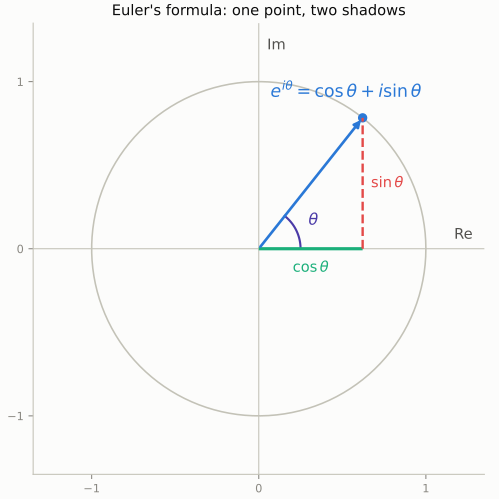
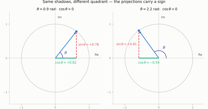
Euler's formula: a point on the unit circle with its cosine and sine projections

One subtlety in this picture is worth pausing on, because it trips people up (it tripped me up): $\cos\theta$ and $\sin\theta$ are signed coordinates, not lengths of a triangle. In the first quadrant the picture looks like ordinary right-triangle trigonometry, and it's tempting to read the two dashed segments as positive side lengths. But push $\theta$ past $\pi/2$ and the horizontal shadow now points in the negative real direction — the triangle looks the same, while $\cos\theta$ has quietly flipped sign:

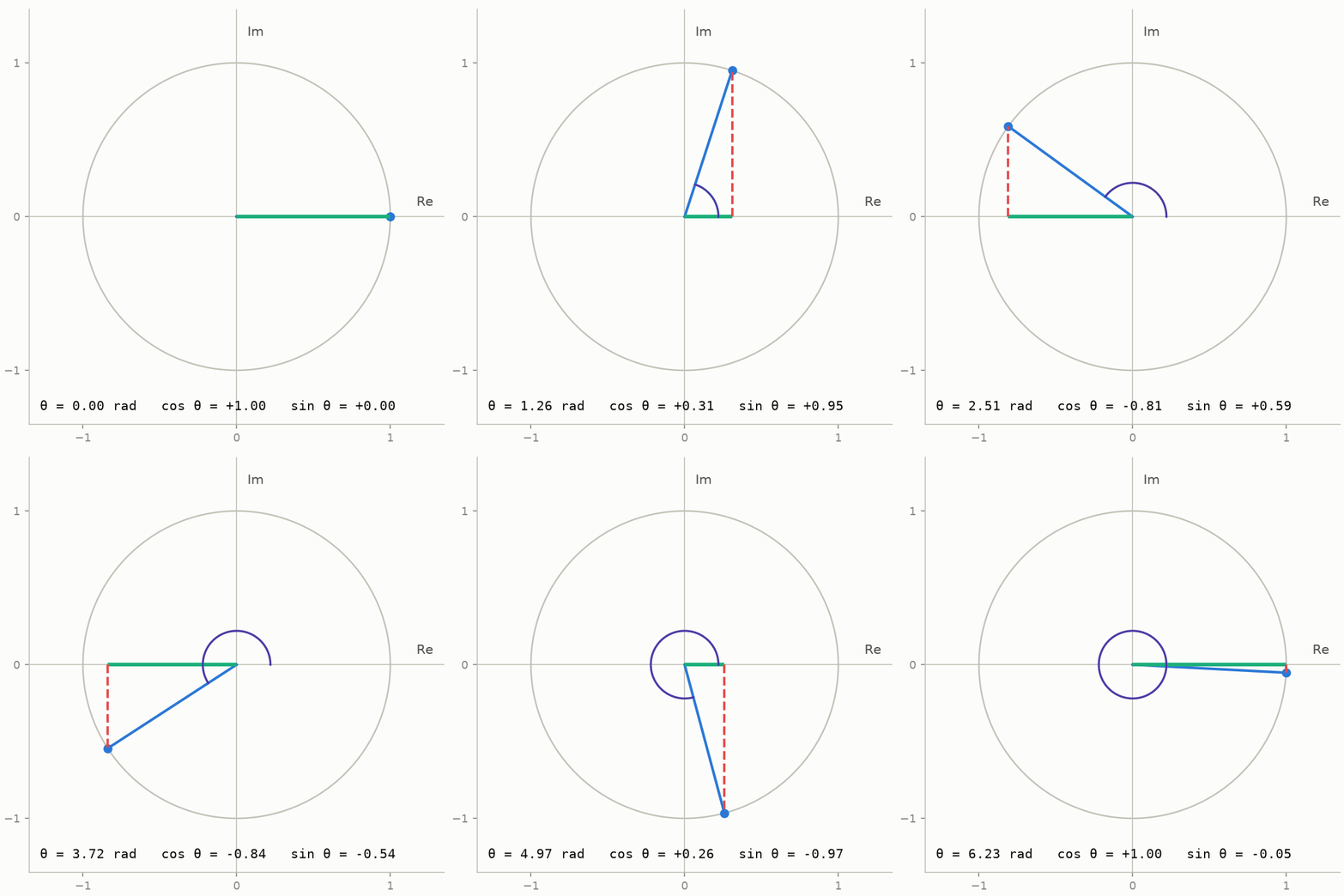
The same construction at two angles: in the second quadrant the cosine projection is negative

Sweeping $\theta$ all the way around makes the bookkeeping obvious — each projection changes sign exactly when the point crosses the corresponding axis, which is precisely why cosine and sine oscillate between $+1$ and $-1$ rather than being humps of positive "length":

θ sweeping the full circle, with the signed cosine and sine projections updating live

Set $\theta = \pi$ and the point lands at $-1$, giving the poster identity $e^{i\pi} + 1 = 0$. But the working form, the one we'll use constantly, is $\theta = \omega t$: a point moving around the circle at constant angular speed $\omega$. Watch its vertical shadow and you get a sine wave; the horizontal shadow is a cosine:

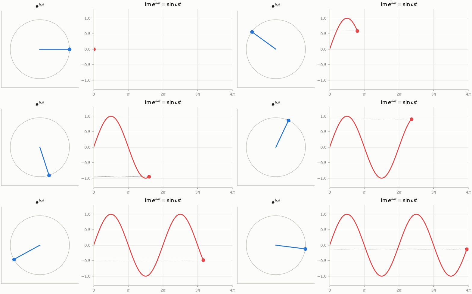
A rotating phasor whose vertical projection traces out a sine wave

This is the fundamental dictionary entry: uniform circular motion ↔ sinusoidal oscillation. A "frequency" is a rotation rate. Everything the Fourier transform does is bookkeeping over a collection of these rotating points, called phasors.

Negative frequency isn't mysterious

In three dimensions — time along one axis, the complex plane in cross-section — the function $e^{it}$ is a helix. Cosine and sine are what you see when you flatten the helix against the floor or the back wall:

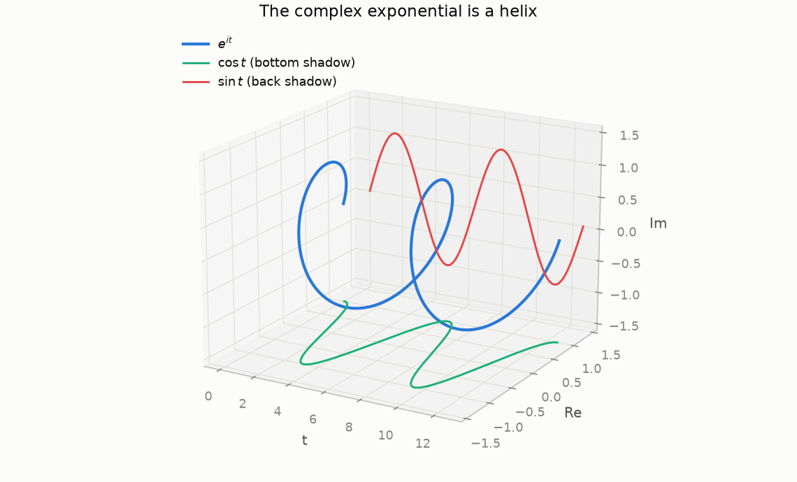
The complex exponential drawn as a helix, with cosine and sine as its projections

A helix has a handedness, and that is all a negative frequency is: $e^{-i\omega t}$ spins clockwise where $e^{i\omega t}$ spins counterclockwise. A real signal has no handedness to prefer, so it must carry both rotations in equal measure. That is the content of the identity

$$ \cos\omega t = \frac{e^{i\omega t} + e^{-i\omega t}}{2}, $$

which says a real oscillation is two counter-rotating phasors whose imaginary parts cancel. When you later see the spectrum of a real signal come out symmetric — every spike at $+\omega$ mirrored at $-\omega$ — this is why. Nothing is "vibrating backwards in time"; the two half-amplitude rotations simply conspire to keep the sum real.

Fourier series: projection onto rotations

Fourier's claim, in modern dress: a reasonable periodic function $f$ with period $2\pi$ can be written as

$$ f(t) = \sum_{n=-\infty}^{\infty} c_n\, e^{i n t}, \qquad c_n = \frac{1}{2\pi} \int_0^{2\pi} f(t)\, e^{-i n t}\, dt . $$

The formula for $c_n$ is not pulled from a hat. The complex exponentials are orthogonal on the interval:

$$ \frac{1}{2\pi}\int_0^{2\pi} e^{i n t}\, \overline{e^{i m t}}\, dt = \begin{cases} 1 & n = m \\ 0 & n \neq m \end{cases} $$

so they behave exactly like perpendicular unit vectors, and $c_n$ is an ordinary dot product — the component of $f$ along the direction $e^{int}$. Fourier analysis is linear algebra in a space where the "vectors" are functions and the orthonormal basis is the family of rotation rates. That framing is worth internalizing now, because in part 2 the integral becomes a finite sum, the basis becomes genuinely finite, and the whole thing becomes a literal matrix.

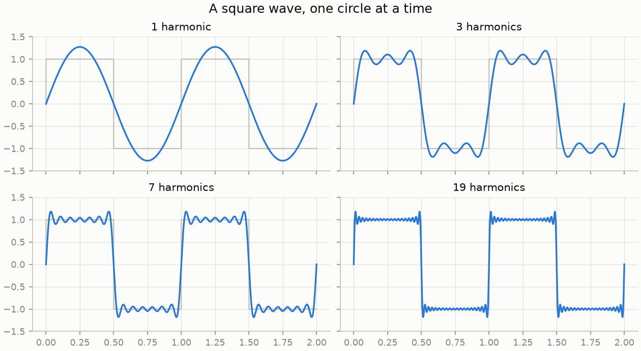
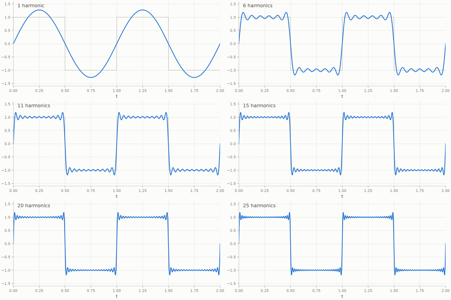
For a square wave the integrals come out to odd harmonics with $1/n$ amplitudes:

$$ \mathrm{square}(t) = \frac{4}{\pi}\left(\sin t + \frac{\sin 3t}{3} + \frac{\sin 5t}{5} + \cdots\right). $$

Here is that sum converging, first as snapshots, then as an animation:

Partial sums of the square-wave Fourier series with 1, 3, 7, and 19 harmonics

Harmonics accumulating one at a time into a square wave

Lagrange's skepticism deserves one concession. Zoom in on the jump and you find the partial sums always overshooting by about 9% of the jump height. Adding more terms squeezes the overshoot into a narrower sliver but never shrinks its height — the Gibbs phenomenon. The series converges at every point, yet not uniformly near the discontinuity:

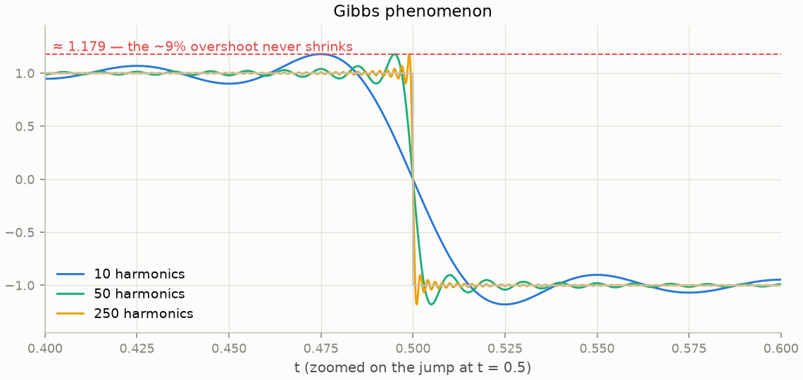
Gibbs phenomenon: the overshoot near the jump stays at about 9% no matter how many harmonics are used

The overshoot lands at $\frac{2}{\pi}\int_0^\pi \frac{\sin s}{s}\,ds \approx 1.179$ for a jump from $-1$ to $1$. This isn't a numerical artifact; it will come back in part 3 as a genuine argument for wavelets, which handle jumps far more gracefully.

Epicycles: the series you can watch

Each term $c_n e^{int}$ is a phasor: a stick of length $|c_n|$ rotating at rate $n$. The series says: chain the sticks tip-to-tail and the end of the chain traces the function. For the square wave, six circles already do a passable job:

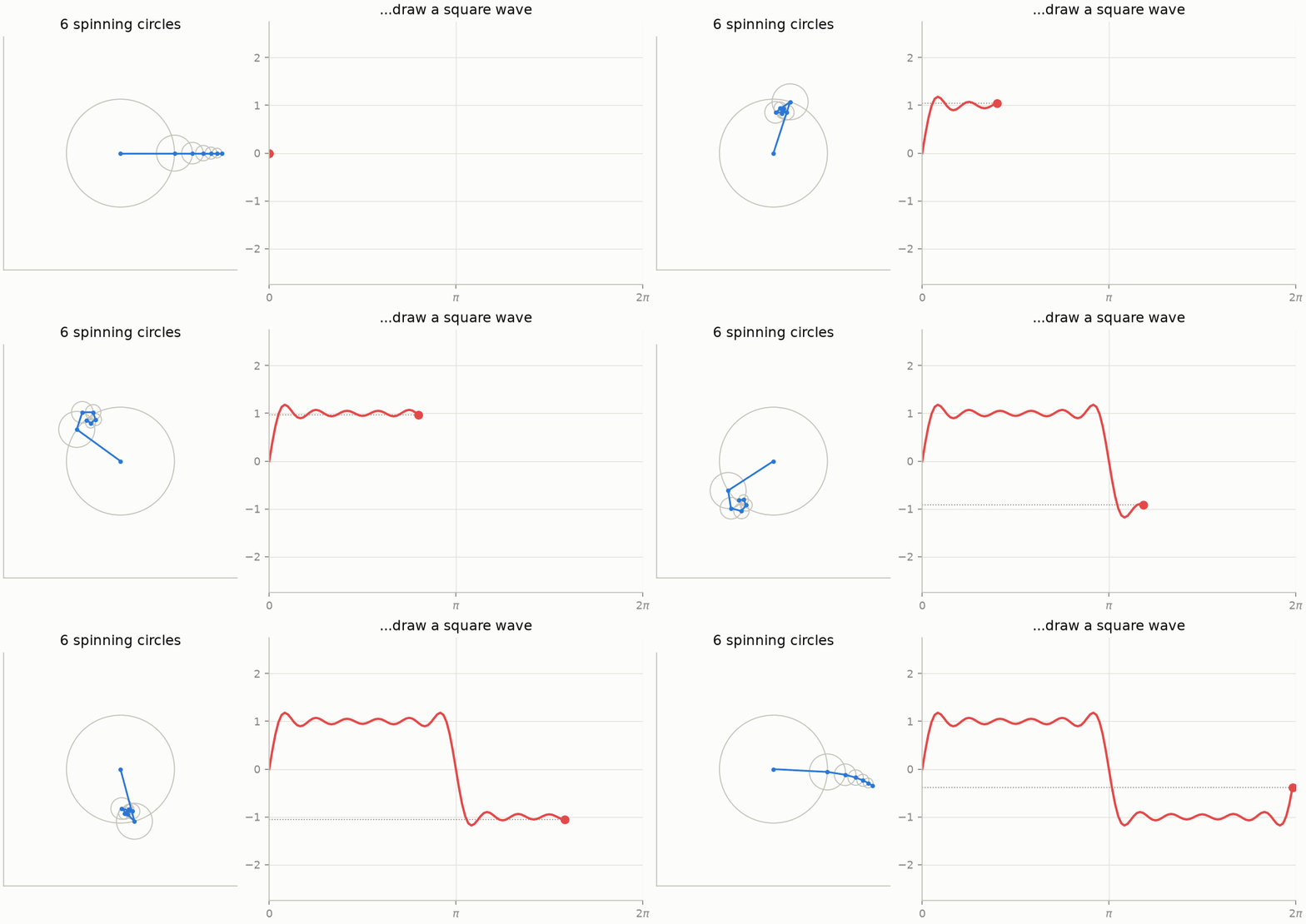
Six chained rotating circles tracing out a square wave

This is Ptolemy's machinery pointed at a waveform instead of a planet — and it's honest mathematics, not just a pretty picture. The largest circle is the fundamental; each smaller, faster circle is a correction term. (The same construction with complex coefficients traces closed curves in the plane, which is how those "draw anything with epicycles" animations work: sample the outline, compute the coefficients — by the end of part 2 you'll know the fast way — and chain the phasors.)

Why sines? Ask the heat equation

One question remains from 1807: why would sines and cosines be the natural currency for heat, of all things? The heat equation on a ring is

$$ \frac{\partial u}{\partial t} = \nu\, \frac{\partial^2 u}{\partial x^2}, $$

and the answer is that complex exponentials are eigenfunctions of the operator $\partial^2 / \partial x^2$: differentiating $e^{ikx}$ twice just multiplies it by $-k^2$. So if you expand the initial temperature in Fourier modes, $u(x, 0) = \sum_k c_k e^{ikx}$, the equation stops coupling anything to anything — each mode evolves alone, by an ordinary one-line ODE, and

$$ u(x, t) = \sum_k c_k\, e^{-\nu k^2 t}\, e^{i k x}. $$

The factor $e^{-\nu k^2 t}$ is the whole story of diffusion: every mode decays exponentially, and the rate grows with the square of the frequency. Wiggles die fast; broad features linger. Watch a jagged temperature profile smooth itself out while its spectrum collapses from the high end:

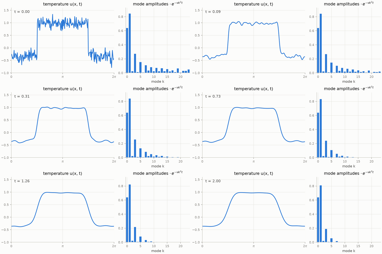
A jagged temperature profile smoothing out as its high-frequency modes decay

This is why Fourier invented the series: the right basis turns a partial differential equation into a family of independent, trivially solvable ordinary ones. Diagonalize the operator, and the physics falls apart into non-interacting pieces. That single move — change to the basis where your operator is diagonal — is the through-line of this series. In part 2 it becomes the FFT and spectral methods; in part 3, the "diagonalize, act, transform back" pattern returns with learned weights in the middle, as a neural operator.

One idea, rediscovered everywhere

There is a final historical point worth making, because it's the best argument I know for the "unreasonable effectiveness" of applied mathematics. Fourier's decomposition wasn't invented once — nature kept forcing it on people who were looking at completely different problems:

Astronomy. Ptolemy's epicycles are a finite Fourier series for a periodic orbit, arrived at ~1,700 years early by fitting circles to the sky. Modern astronomy still runs on the same mathematics — radio interferometers like the VLA and the Event Horizon Telescope measure the Fourier transform of the sky's brightness directly, and reconstruct the image from it.
Crystallography. When X-rays scatter off a crystal, the diffraction pattern on the detector is the Fourier transform of the electron density. Solving a structure — including DNA's — is literally the problem of inverting a Fourier transform whose phases were lost in measurement.
Chemistry and medicine. An FT-NMR spectrometer hits nuclei with a pulse and records the decaying echo; the spectrum is its Fourier transform. Richard Ernst won the 1991 Nobel Prize in Chemistry for realizing this beats scanning frequencies one at a time — and MRI reconstructs images from exactly the same k-space mathematics.
Physics. LIGO finds gravitational waves by matched filtering — correlating the strain data against template waveforms, computed as products in the frequency domain because convolution is cheap there. (That convolution theorem is the centerpiece of part 2.)
Computational fluids. Spectral methods solve the Navier–Stokes equations by evolving Fourier coefficients instead of grid values — the standard tool for simulating turbulence, and the direct ancestor of the neural operators in part 3.
Your screen. JPEG and most video codecs quantize the discrete cosine transform — a real-valued cousin of the DFT — throwing away the high-frequency coefficients your eye won't miss.

None of these fields set out to do "Fourier analysis." Each found that its signals, when written in the basis of oscillations, became simple — because waves, diffusion, and periodic motion are what the physical world is made of, and this is the basis that diagonalizes them. That is the recurring miracle of applied math: a representation invented to settle an argument about heat turns out to be something nature had already committed to.

Where this goes

Part 2 discretizes: the Fourier series becomes the DFT (a matrix), the FFT makes it fast, and the convolution theorem plus spectral derivatives make it useful — with detours through sampling, aliasing, and what a spectrogram of an actual song looks like. Part 3 covers what Fourier can't do — localize in time and frequency at once — and follows wavelets to a modern endpoint: wavelet neural operators, trained in JAX on Burgers' equation.

Table of Contents