Table of Contents
Why this exists
Improper payments and vendor fraud are persistent risks in public-finance
operations, and review capacity is always limited. This project is a
prototype payment-integrity risk scoring system: it takes a single
payment transaction, scores it for fraud/payment-integrity risk in [0, 1],
assigns a low / medium / high risk level, and produces a short list of
human-readable reasons for that score. The model recommends; a human
decides -- nothing is automatically blocked, approved, or reported.
Everything in this article is computed on synthetic data only. No real vendor, payment, or personal information is used anywhere. The point of the prototype is to demonstrate a complete, auditable pipeline -- data generation, feature engineering, training, evaluation, and serving -- with every modeling choice documented and, where relevant, derived from first principles.
Architecture at a glance
flowchart LR
    subgraph TRAIN["Training (pixi run train)"]
        DG["Synthetic data generation"] --> FE["Feature engineering"]
        FE --> CLS["JAX logistic regression\n(supervised classifier)"]
        FE --> AD["IsolationForest\n(anomaly detector)"]
        DG --> GRAPH["Vendor relationship graph\n(shared bank account / address)"]
        GRAPH --> DIFF["Learned diffusion operator\n(resolvent + conjugate gradient,\njointly fine-tuned with classifier)"]
        CLS -.-> DIFF
        DIFF --> ARTIFACT["vendor_graph_features.json"]
    end

    subgraph SERVE["Serving"]
        ARTIFACT --> LOOKUP["graph_diffusion_risk_score\nlookup by vendor_id"]
        CLS --> COMBINE["Combined risk score"]
        AD --> COMBINE
        LOOKUP --> COMBINE
        COMBINE --> RULES["Risk-level rules\n+ explanations"]
        RULES --> API["FastAPI /predict"]
        RULES --> DASH["Streamlit dashboard"]
    end
Two models feed a combined score:
-
A JAX logistic regression classifier, trained on a class-weighted, L2-regularized binary cross-entropy loss:
$$ \mathcal{L}(w, b) = \frac{1}{n}\sum_{i=1}^n c_i\big[-y_i\log\hat p_i - (1-y_i)\log(1-\hat p_i)\big] + \lambda \lVert w \rVert_2^2, \qquad \hat p_i = \sigma(x_i^\top w + b) $$
The per-example weight $c_i$ is $n/(2n_{\text{pos}})$ for fraud rows and $n/(2n_{\text{neg}})$ for non-fraud rows, so the ~5% fraud class contributes as much to the gradient as the ~95% non-fraud class -- class-weighting instead of resampling. Trained with $\eta=0.05$, $\lambda=10^{-4}$, 500 full-batch gradient-descent epochs.
-
A scikit-learn IsolationForest anomaly detector on the same scaled feature matrix, catching transactions that look statistically unusual even if the classifier assigns them a low fraud probability. Its raw score is min-max normalized to
[0, 1]over the training set. -
A combined risk score:
$$ \texttt{fraud_risk_score} = \mathrm{clip}\big(0.75,p_{\text{clf}} + 0.25,a,\ 0,\ 1\big) $$
with risk levels
low(< 0.35),medium(0.35-0.70),high(>= 0.70). -
Independent, rule-based explanations (
top_risk_factors) -- e.g. "vendor is newly created", "duplicate invoice score is high" -- so the human-readable reasons stay stable and interpretable regardless of how the underlying model weights change.
Two of the 20 input features are themselves small statistical models rather than raw inputs:
$$ \texttt{amount_zscore_vs_vendor_avg} = \frac{\texttt{transaction_amount} - \texttt{avg_vendor_amount_90d}} {\max(\texttt{vendor_amount_std_90d},\ 1)} $$
$$ \texttt{payment_frequency_ratio} = \frac{\texttt{num_payments_vendor_30d}} {\max(\texttt{vendor_avg_monthly_txn_count},\ 0.1)} $$
i.e. how many standard deviations the current transaction is from this vendor's historical average, and how the recent 30-day payment count compares to this vendor's typical monthly count.
How well does it work?
On a held-out test split of 2,000 synthetic transactions (5.1% fraud rate):
| Metric (classifier only) | Value |
|---|---|
| ROC AUC | 0.839 |
| Average precision (PR AUC) | 0.334 |
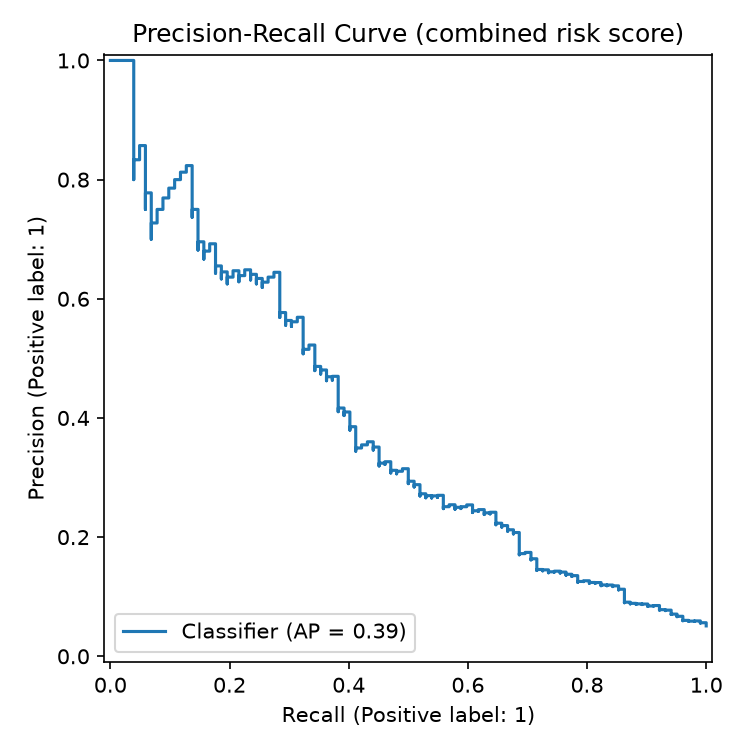
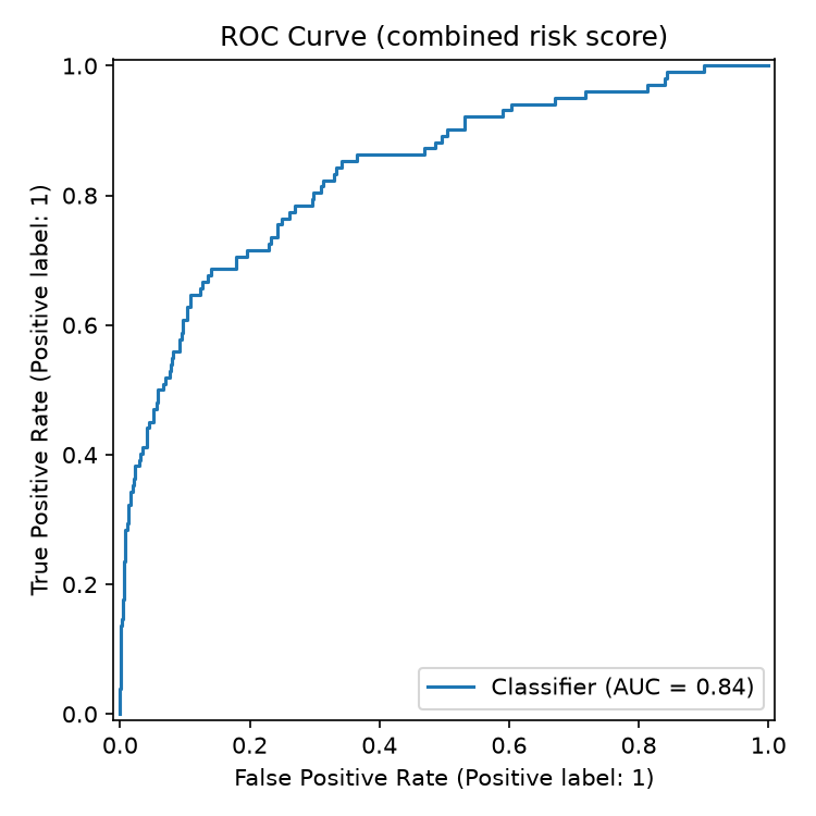
| Metric (combined: classifier + anomaly) | Value |
|---|---|
| ROC AUC | 0.838 |
| Average precision (PR AUC) | 0.387 |
| Threshold | Accuracy | Precision | Recall | F1 |
|---|---|---|---|---|
| 0.35 (low/medium boundary) | 0.697 | 0.123 | 0.804 | 0.213 |
| 0.50 | 0.846 | 0.202 | 0.686 | 0.312 |
| 0.70 (medium/high boundary) | 0.932 | 0.353 | 0.412 | 0.380 |
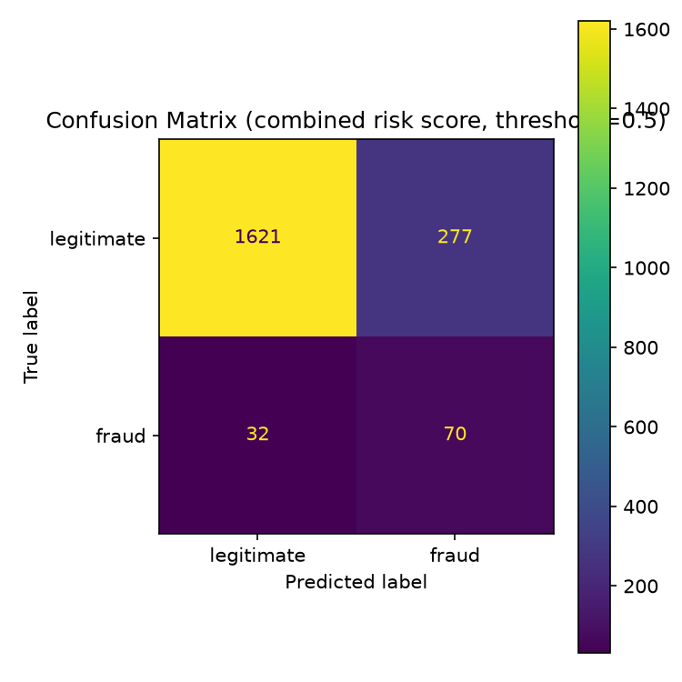
Reading these numbers: at the low/medium boundary the model catches
~80% of fraud in the synthetic test set but flags ~35% of all transactions --
exactly the shape you want from a screening tool whose job is to widen the
pool for human review, not to make a final call. At the medium/high
boundary, roughly 1 in 3 transactions flagged high is actually fraud in the
synthetic labels; for a rare event at a 5.1% base rate, that's the expected
precision/recall trade, which is why a human reviewer -- not an automated
action -- sits at the end of the pipeline.
Is logistic regression leaving anything on the table?
To check whether the simple, fully-auditable linear model is competitive, three scikit-learn/XGBoost baselines were trained on the same train/test split and the same fitted feature scaler:
| Model | ROC AUC | Average Precision |
|---|---|---|
| JAX logistic regression (served) | 0.839 | 0.334 |
| scikit-learn logistic regression | 0.840 | 0.333 |
| Random forest | 0.850 | 0.386 |
| XGBoost | 0.840 | 0.355 |
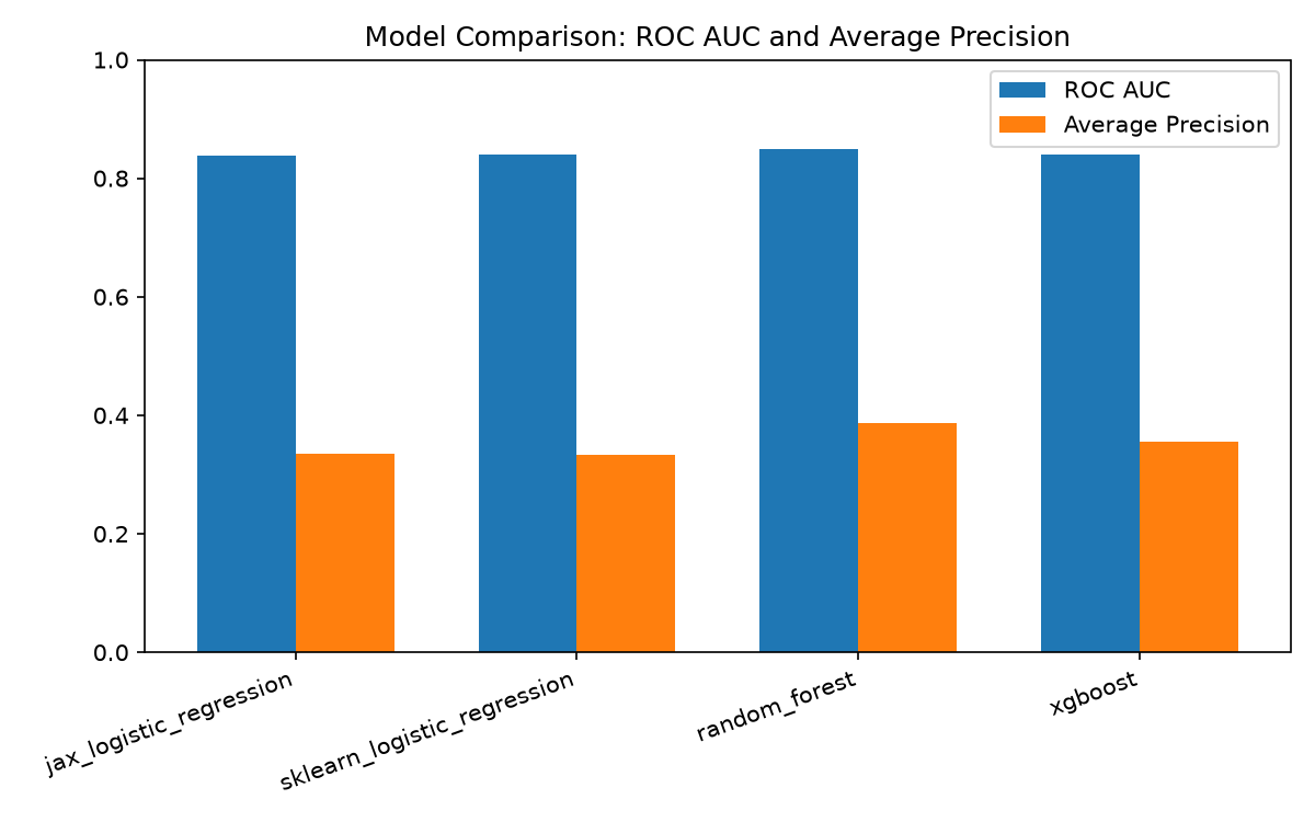
Random forest leads on both metrics, but the gap (ROC AUC 0.839 vs. 0.850) is modest, and the JAX logistic regression is nearly identical to the scikit-learn baseline that fits (almost) the same linear decision boundary on the same features -- as expected. The served model stays the simple linear one: the gap isn't large enough to trade away an end-to-end auditable training and inference path. A small JAX MLP is the natural next step if closing that gap becomes a priority.
The interesting part: graph diffusion as "guilt by association"
Most of the 20 input features describe a transaction or a vendor in
isolation. One feature, graph_diffusion_risk_score, instead describes a
vendor's position in a network.
Building the vendor graph
Vendors that share a bank account or a mailing address are connected in an undirected, edge-weighted graph. For identifier type $k \in {\text{bank}, \text{addr}}$, every pair of vendors sharing identifier value $v$ of type $k$ gets edge weight $w_k / (m_k(v) - 1)$, where $m_k(v)$ is the size of the group sharing that value:
$$ W_{ij} = \sum_{k\in{\text{bank},,\text{addr}}} \frac{w_k\cdot \mathbb{1}[i\ne j,\ i,j\text{ share identifier }k]}{|\text{group sharing that identifier}| - 1} $$
This rarity normalization is the key design choice: each vendor's total connection strength via identifier type $k$ is exactly $w_k$, whether it shares that identifier with 1 other vendor or 50. A common address shared by 20 vendors doesn't become a diffusion "shortcut" relative to a rare shared bank account. A shared bank account ($w_{\text{bank}}=1.0$) is also weighted more heavily than a shared address ($w_{\text{addr}}=0.5$), encoding "a shared bank account is a stronger signal."
Spreading risk: the resolvent
Start from a seed vector $s$: $1$ for vendors with confirmed prior flags
(prior_vendor_flags >= 2), $0$ everywhere else. The diffused score solves
the regularized graph Laplacian resolvent:
$$ (I + \beta L)x = s, \qquad L = D - W $$
solved via conjugate gradient, where $D = \mathrm{diag}(W\mathbf{1})$ is the weighted degree matrix. This is the steady state of a reaction-diffusion equation $\dot x = -Lx - \gamma(x - s)$ with $\beta = 1/\gamma$: diffusion ($-Lx$) spreads risk along edges, while the reaction term continuously re-injects each vendor toward its own seed value. $x$ is the regularized Laplacian kernel (closely related to personalized PageRank) -- a standard "graph diffusion with restart" construction.
Both the maximum principle ($\min_j s_j \le x_i \le \max_j s_j$ for every
$i$, for any $\beta \ge 0$) and mass conservation ($\sum_i x_i = \sum_i s_i$)
hold for this resolvent, so the score stays bounded in [0, 1] and every
vendor's elevated score is fully explained by risk mass elsewhere in its
connected component.
$\beta$ is a spectral low-pass filter
Diagonalizing $L = U\Lambda U^\top$:
$$ (I+\beta L)^{-1} = U,\mathrm{diag}!\left(\frac{1}{1+\beta\lambda_k}\right)U^\top $$
Each eigenmode of the seed is attenuated by $\frac{1}{1+\beta\lambda_k} \in (0, 1]$, monotonically decreasing in both $\lambda_k$ and $\beta$, with no stability constraint on $\beta$ -- unlike a fixed-step explicit-Euler diffusion scheme, where too large a step size makes the filter oscillate in sign. $\beta \to 0$ recovers the raw seed; $\beta \to \infty$ collapses every vendor in a component to that component's mean seed value.
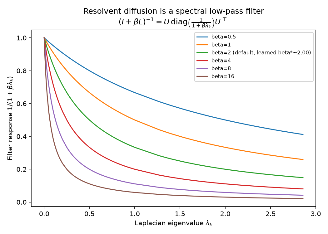
This single plot is the whole design rationale: pick a $\beta$ that sits between "no diffusion" and "everyone in a component looks the same."
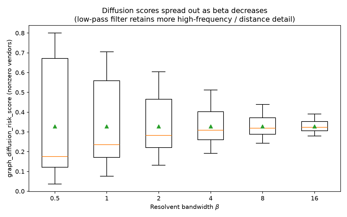
What this does to the actual scores
Plotting the nonzero graph_diffusion_risk_score values across a sweep of
$\beta$ shows exactly the predicted effect -- smaller $\beta$ keeps more
high-frequency (i.e. distance-sensitive) detail, so scores spread out instead
of clustering in a narrow band:
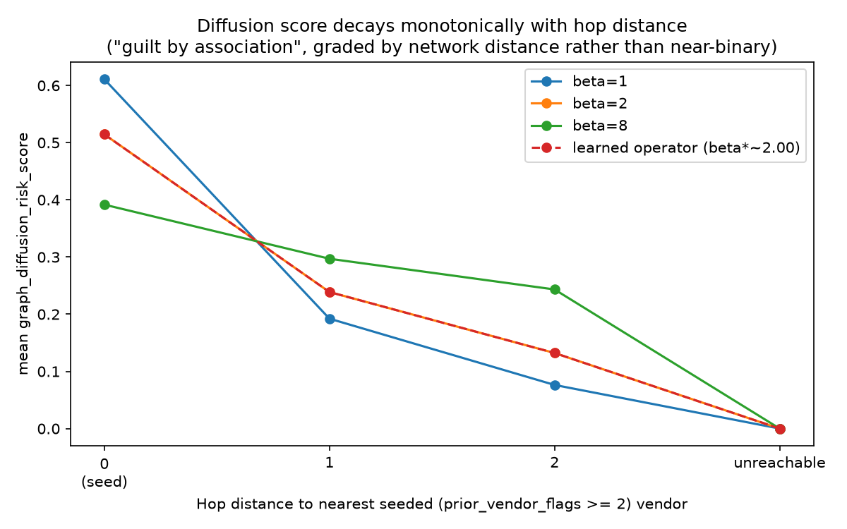
And the score decays monotonically with hop distance from the nearest
flagged vendor -- vendors directly sharing an identifier with a flagged vendor
score highest, vendors two hops away score lower, and vendors with no path to
any flagged vendor score exactly 0:
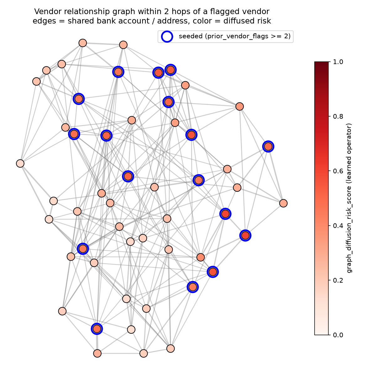
Here's the actual subgraph this is computed on -- every vendor within two hops of a flagged vendor, colored by its diffused risk score:
Making $\beta$ (and the edge weights) learnable
The bandwidth $\beta$ and the per-identifier-type weights $w_{\text{bank}}$,
$w_{\text{addr}}$ don't have to be fixed constants. Reparameterized through
softplus to stay positive --
$\beta=\mathrm{softplus}(\theta_\beta)$,
$w_{\text{bank}}=\mathrm{softplus}(\theta_{\text{bank}})$,
$w_{\text{addr}}=\mathrm{softplus}(\theta_{\text{addr}})$ -- these three
scalars are fine-tuned jointly with the classifier weights, by
differentiating through the conjugate-gradient solve itself
(jax.scipy.sparse.linalg.cg is differentiable; because $I+\beta L$ is
self-adjoint, the backward pass is just another CG solve with the same
matrix). This is a tiny, physically-structured "neural operator" -- three
learned scalars governing a well-understood linear operator, not a black-box
graph neural network.
Training starts from the 0.3.1 fixed defaults ($\beta=2.0$,
$w_{\text{bank}}=1.0$, $w_{\text{addr}}=0.5$) and, for this dataset/seed,
barely moves: $\beta^\approx 1.99993$, $w^{\text{bank}}\approx 0.99954$,
$w^*{\text{addr}}\approx 0.50030$. Because the score now depends on the
trained operator, it can no longer be precomputed at data-generation time --
train.py computes final per-vendor scores over the full vendor graph and
writes a vendor_graph_features.json lookup (vendor_id -> score, plus a
cold-start default), which the API, evaluation, model comparison, and
dashboard all read consistently.
Takeaways
- A linear classifier plus an anomaly detector plus a handful of interpretable, hand-derived features gets to ROC AUC ~0.84 on this synthetic task -- and stays fully auditable end to end.
- The graph diffusion feature turns "is this vendor connected to a known bad
actor?" into a graded
[0, 1]signal with provable bounds (maximum principle, mass conservation), governed by a single, stability-free bandwidth parameter with a clean spectral interpretation. - That bandwidth -- along with the relative weight of "shared bank account" vs. "shared address" -- can be learned end-to-end alongside the classifier, while still being just three scalars controlling a well-understood linear operator.
All of the numbers and plots above are reproducible from a fixed random seed:
pixi run generate-data
pixi run train
pixi run evaluate
pixi run compare-models
pixi run analyze-graph-diffusion
See the project README and docs/model_card.md for the full model card,
threat model, and risk assessment.